Aircraft Stability & Control Simulation

Role

Team Member — Stability Analysis & Simulation

AE 413: Aircraft Stability and Control · ERAU · Spring 2025

Tools

MATLAB · Simulink · USAF DATCOM · FlightGear
Multhopp’s Theory · Hand Calculations

Key Contributions

Designed original aircraft geometry (22 ft span, 121 ft² wing area, AR = 4) from scratch using class-derived sizing requirements
Computed longitudinal, directional, and lateral stability derivatives both analytically and via USAF DATCOM, achieving <3.5% error on C_nβ and C_lβ
Integrated five DATCOM lookup-table derivatives into a Simulink 6-DOF flight dynamics model with FlightGear visualization
Verified static stability (neutral point at 43.5% MAC) and confirmed positive directional and lateral stability margins

This page walks through a clean-sheet aircraft stability and control study — from geometry sizing and hand-derived stability derivatives, through DATCOM cross-validation, to a closed-loop 6-DOF Simulink model visualized live in FlightGear.

Project Overview

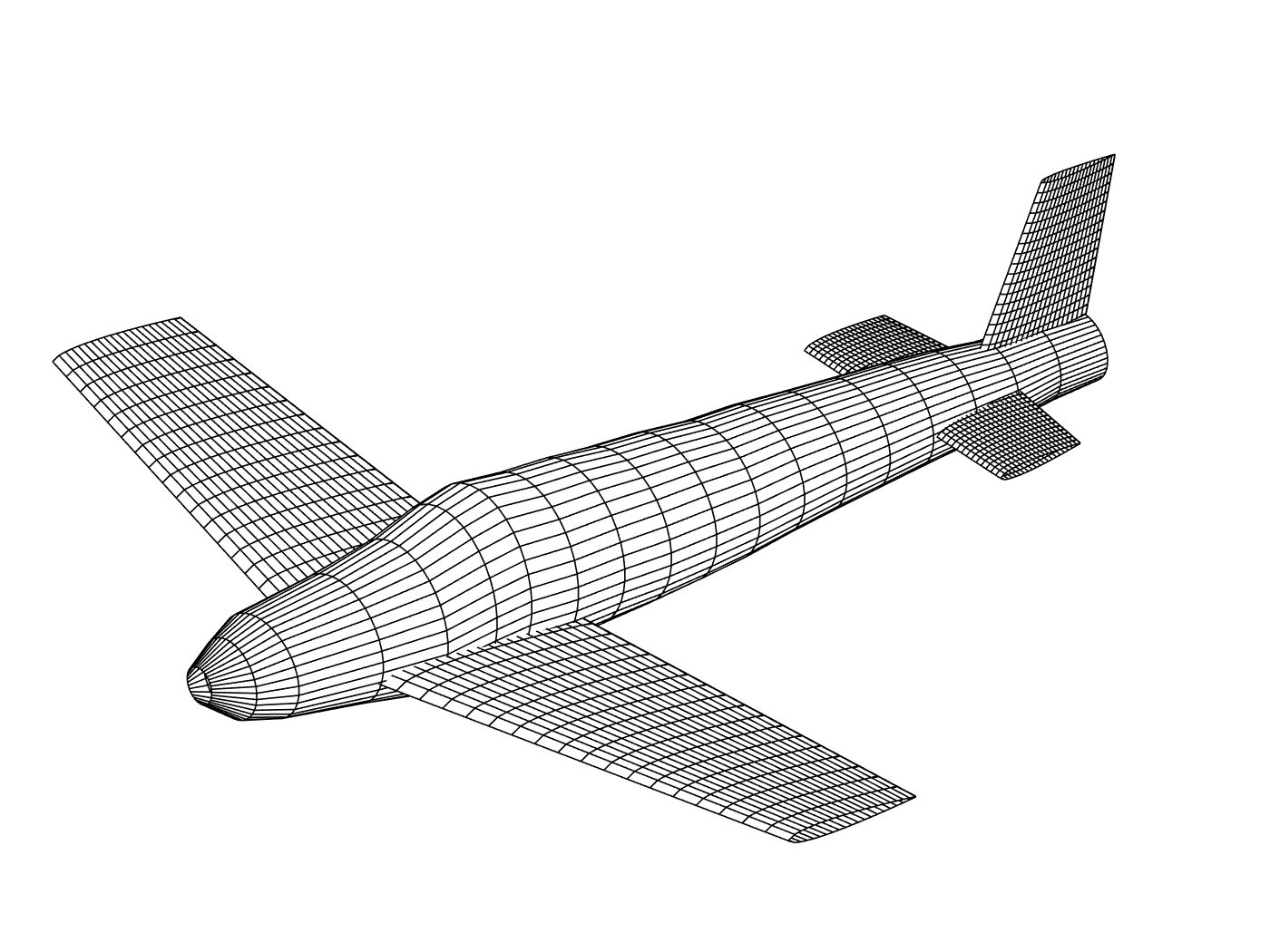
This project covered the full cycle of aircraft stability and control analysis — from geometry sizing and hand-derived stability derivatives all the way through closed-loop simulation and 3D flight visualization. The aircraft was a clean-sheet design, sized to fly at Mach 0.6 and 6,500 ft altitude at a trimmed angle of attack of 2°, carrying two passengers at a gross weight of 4,000 lb. The goal was to demonstrate that a designed configuration could simultaneously satisfy aerodynamic, geometric, and stability requirements, and then validate that behavior computationally.

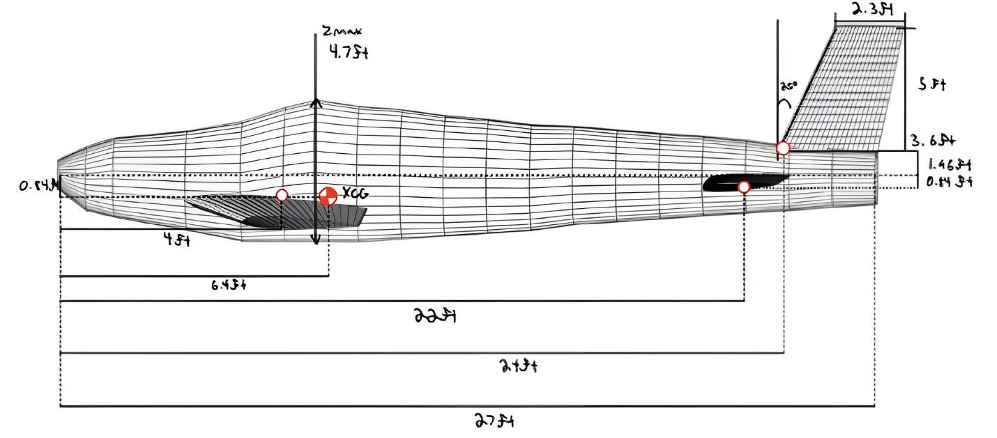
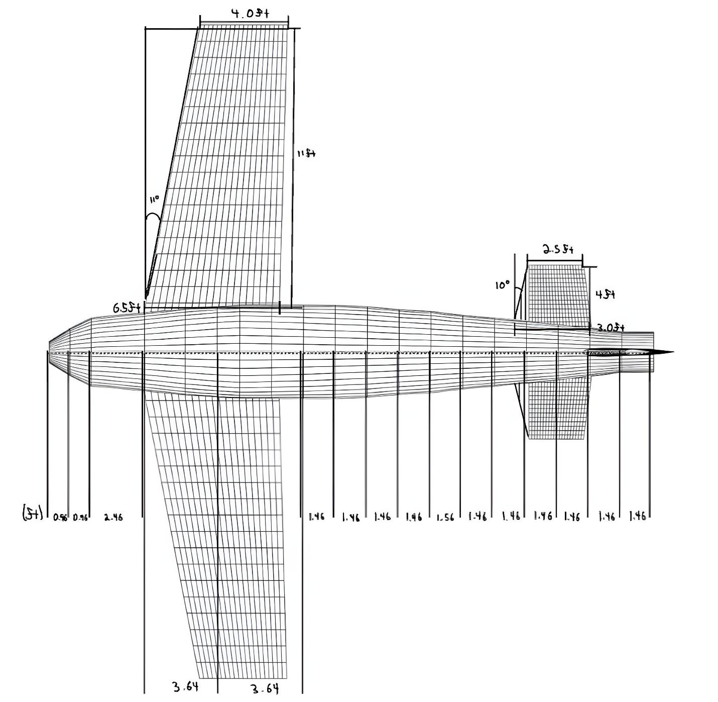
Define aircraft geometry (wing, horizontal tail, vertical tail, fuselage) to satisfy required C_Lα, C_D0, C_mα, and C_nβ targets
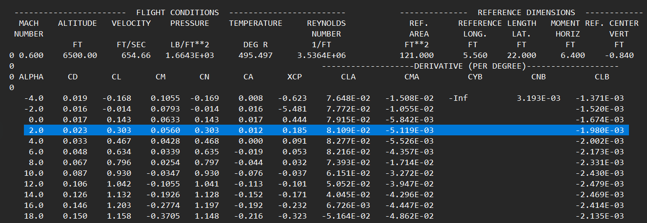
Compute key stability derivatives analytically and cross-validate with USAF DATCOM across multiple flight conditions and angles of attack
Integrate five dynamic derivatives (C_nr, C_np, C_mq, C_lα, C_nb) as lookup-table blocks in a Simulink 6-DOF general aviation model
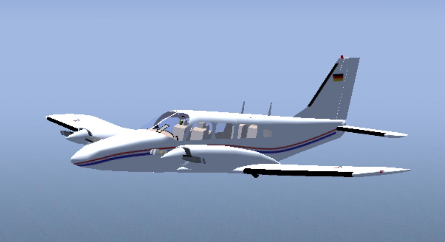
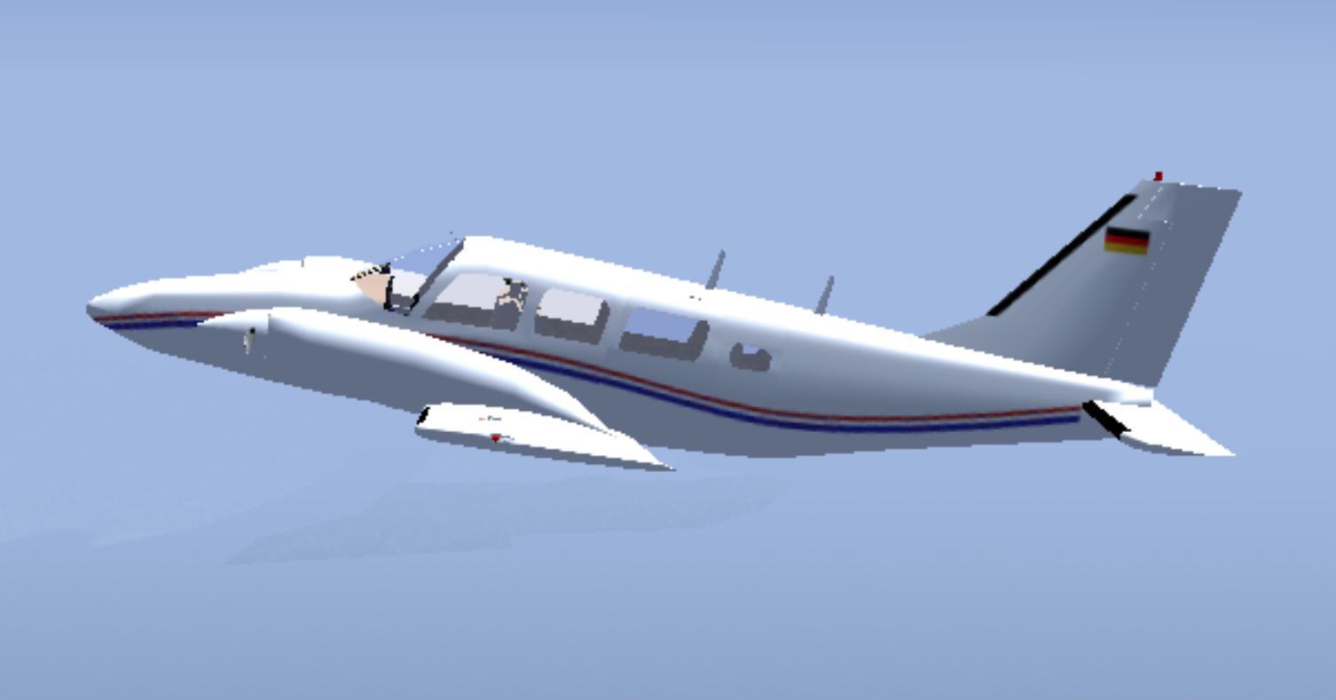
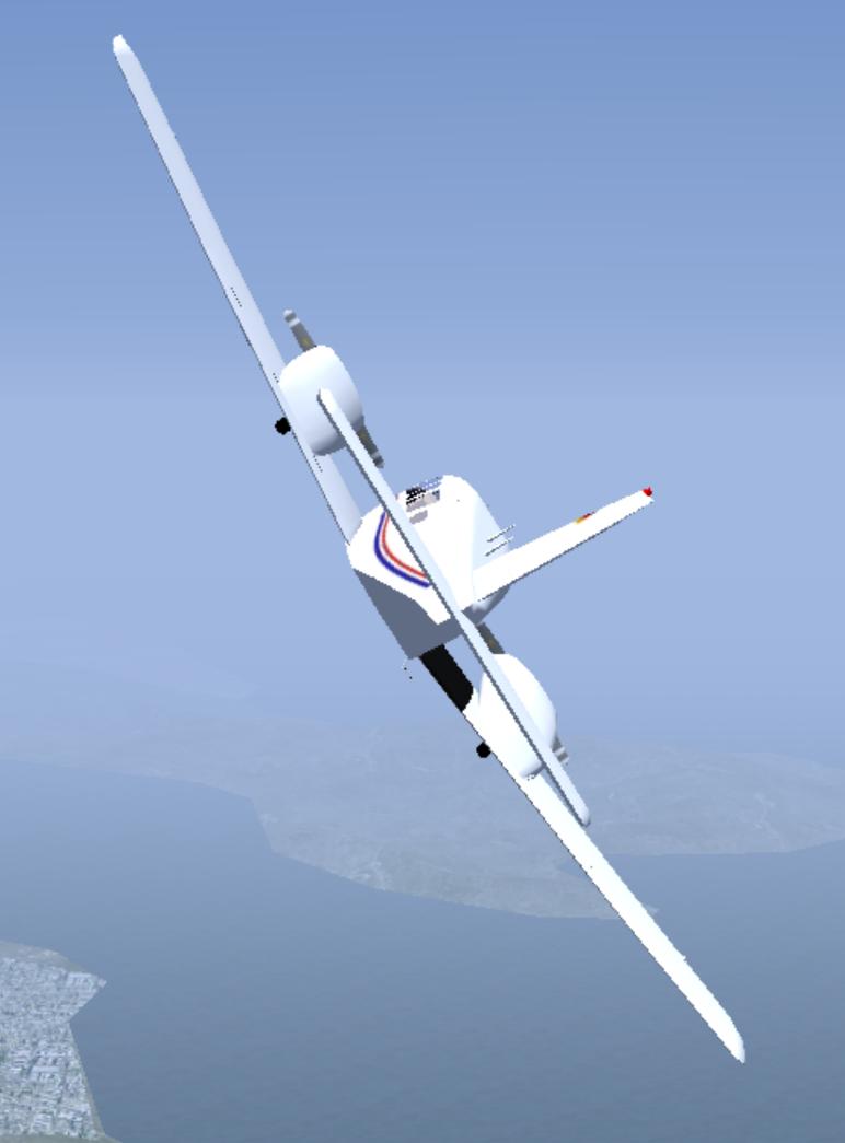
Visualize level flight, pitch-up, and right-bank maneuvers through the FlightGear flight simulator interface

MATLAB 3D wireframe orthogonal view of designed aircraft — Fig. 1: MATLAB 3D wireframe model (orthogonal view) of the designed aircraft, generated using the DATCOM 3D visualization code. Wingspan: 22 ft, fuselage length: 27.7 ft.

Aircraft Geometry & Design Parameters

The aircraft configuration was established through manual geometric sizing. Wing parameters were selected to hit the required lift-curve slope and longitudinal stability margin, while tail sizing was driven by horizontal-tail volume coefficient constraints. The final design used an 11° leading-edge sweep and 3° dihedral on the main wing to balance lateral stability and aerodynamic efficiency.

Parameter	Wing	Horizontal Tail
Root Chord	6.5 ft	3.0 ft
Tip Chord	4.5 ft	2.5 ft
Wingspan / Span	22 ft	8 ft
Wing Area	121 ft²	22 ft²
Mean Aerodynamic Chord	5.561 ft	2.758 ft
Aspect Ratio	4.0	2.909
Sweep Angle	11°	10°
Dihedral Angle	3°	8°
Taper Ratio	0.692	0.833

Key flight-condition parameters and resulting aerodynamic coefficients at α = 2°:

Parameter	Value
Altitude	6,500 ft
Mach Number	0.6
Gross Weight	4,000 lb
Fuselage Length	27.708 ft
C_L0	0.143
C_D0	0.017
C_Lα	4.648 rad⁻¹ (0.0811 deg⁻¹)
C_mα (DATCOM)	−0.293 rad⁻¹
C_nβ	0.183 rad⁻¹
Stall Speed	163.8 ft/s

CAD side view of aircraft with dimensions — Fig. 2: CAD side view with fuselage and wing station dimensions.

CAD top view of aircraft — Fig. 3: CAD top view showing wing sweep, taper, and tail layout.

Longitudinal Stability Analysis

Longitudinal static stability was evaluated through the pitching-moment curve slope C_mα, which must be negative for a statically stable aircraft. The total C_mα is the sum of fuselage, wing, and horizontal-tail contributions. The fuselage contribution was computed using Multhopp’s theory (implemented as a MATLAB script), which integrates the pitching moment over 100 upwash and 100 downwash fuselage cross-sections, yielding C_mα,f = 0.4702 rad⁻¹. Combined with the wing contribution (−0.297 rad⁻¹) and tail contribution (−1.53 rad⁻¹), the hand-calculated total is:

C_mα = 0.4702 − 0.297 − 1.53 ≈ −1.35 rad⁻¹

DATCOM reported C_mα = −0.293 rad⁻¹, a significant departure from the analytical result. Both values are negative, confirming the aircraft is statically stable in pitch, though the magnitude — and therefore the static margin — differs between the two methods. The neutral point was computed analytically at N₀ = 0.435 (43.5% MAC).

Design Decision

Trade-off: Reported both the hand-calculated C_mα (−1.35 rad⁻¹) and the DATCOM value (−0.293 rad⁻¹) side by side rather than reconciling them to a single number.

Why: The discrepancy is attributed to DATCOM’s semi-empirical assumptions, which can underestimate tail effectiveness for certain geometry configurations. Since both methods agree on the sign (statically stable) but disagree on magnitude, presenting both values preserves that information for downstream design decisions rather than masking it with a single averaged figure.

DATCOM output table showing longitudinal stability coefficients — Fig. 4: DATCOM output at Mach 0.6, 6,500 ft. The highlighted row at α = 2° gives C_mα = −0.005119/deg = −0.2943 rad⁻¹.

Hand calculations for downwash model and Cma — Fig. 5: Analytical downwash model computation (dε/dα = 0.456) and breakdown of C_mα by aircraft component.

Directional & Lateral Stability Analysis

Directional stability is characterized by C_nβ (weathercock stability derivative) — a positive value indicates the aircraft yaws nose-into-the-wind when disturbed, which is the required stable behavior. Lateral stability is characterized by C_lβ (dihedral effect) — a negative value means the aircraft rolls away from a sideslip, which is likewise stable. Both were computed analytically, incorporating contributions from the wing, fuselage, and vertical tail.

Directional stability (C_nβ): Hand-calculated 0.189 rad⁻¹ · DATCOM 0.183 rad⁻¹ · error <3.5% — the close agreement confirms the vertical tail is correctly sized for adequate yaw stiffness at this flight condition
Lateral stability (C_lβ): Hand-calculated −0.1231 rad⁻¹ · DATCOM −0.113 rad⁻¹ · difference 0.01 rad⁻¹ — well within acceptable engineering agreement, and both values confirm negative (stable) dihedral effect

The 3° wing dihedral combined with the wing sweep contributes the dominant stabilizing lateral moment.

Hand calculations for directional stability Cnbeta — Fig. 6: Analytical computation of directional stability derivative C_nβ, summing fuselage, wing, and vertical-tail contributions.

Hand Calculations vs. DATCOM — Comparison

The table below summarizes the full derivative comparison at the design point (α = 2°, Mach 0.6, 6,500 ft). Good agreement was achieved for most aerodynamic coefficients. The significant discrepancy in C_mα underscores that DATCOM’s semi-empirical methods have known limitations for tail-effectiveness estimation on configurations where the horizontal tail is a strong contributor to longitudinal stability, warranting cross-verification with analytical methods.

Parameter	Hand-Calculated	DATCOM
C_Lα	0.0741 deg⁻¹	0.08109 deg⁻¹
C_L	0.291	0.303
C_D	0.024	0.023
V_stall	163.8 ft/s	163.8 ft/s
dε/dα	0.456	0.461
C_mα	−1.35 rad⁻¹	−0.293 rad⁻¹
C_nβ	0.189 rad⁻¹	0.183 rad⁻¹
C_lβ	−0.1231 rad⁻¹	−0.113 rad⁻¹
N₀ (Neutral Point)	0.435 (43.5% MAC)	N/A
C_mδe	−0.01385 deg⁻¹	N/A

Simulink Integration & Dynamic Derivatives

Five stability derivatives computed by DATCOM were integrated as 1-D lookup-table (T(u)) blocks in a Simulink 6-DOF general aviation flight dynamics model. Each lookup table maps angle of attack (in degrees) to its respective derivative value, evaluated at the design flight condition. This non-linear aerodynamic representation is more accurate than fixed-derivative linear models because it captures how the derivatives change across the angle-of-attack range from −4° to +18°.

Derivative	Physical Meaning	Value at α = 2°
C_nr	Yaw damping due to yaw rate	−0.008426
C_np	Yaw moment due to roll rate	−0.0006962
C_mq	Pitch damping due to pitch rate	−0.1992
C_lα	Lift-curve slope	0.08109
C_nb	Yaw moment due to sideslip	0.003193

Simulink lookup table blocks for five aerodynamic derivatives — Fig. 7: Simulink 1-D lookup-table blocks for C_nr, C_np, C_mq, C_lα, and C_nb. Display values shown at α = 2°.

Simulink 6-DOF flight dynamics model connected to FlightGear — Fig. 8: Full Simulink flight dynamics model. The DATCOM aerodynamic lookup tables feed the Discrete Time General Aircraft Model block, which outputs 6-DOF states to FlightGear for real-time visualization.

Simulation Results — FlightGear Maneuvers

Three maneuvers were simulated in FlightGear to validate the aircraft’s dynamic behavior and control authority. In each case, Simulink passed state outputs (roll, pitch, yaw, altitude, airspeed) to FlightGear in real time, providing a 3D visual confirmation that the aerodynamic model produces physically plausible responses.

Level Flight · V = 654 ft/s · δ_e = −1.71° · Alt = 6,500 ft — the −1.71° elevator deflection trims the aircraft at the design point. The negative sign indicates the elevator must be deflected trailing-edge-up (download on the tail) to maintain 2° angle of attack — consistent with a statically stable, aft-CG aircraft
Pitch-Up · V = 630 ft/s · δ_e = +2° · Alt = 6,530 ft — produces a nose-up pitch response and a modest altitude gain of ~30 ft, confirming positive elevator effectiveness (negative C_mδe). The slight airspeed decrease to 630 ft/s is physically consistent with the pitch-altitude energy exchange
Right Bank · V = 654 ft/s · all surfaces neutral · Alt = 6,500 ft — demonstrates the model’s lateral-directional dynamics. With neutral controls, any induced roll couples through the dihedral effect (C_lβ = −0.113 rad⁻¹) and directional stability (C_nβ = 0.183 rad⁻¹) to produce the characteristic spiral and Dutch-roll coupling inherent to the design

FlightGear level flight simulation screenshot — Fig. 9: Level flight at 6,500 ft. Elevator = −1.71° for trim.

FlightGear pitch-up maneuver simulation screenshot — Fig. 10: Pitch-up at δ_e = +2°; aircraft climbs to 6,530 ft.

FlightGear right bank maneuver simulation screenshot — Fig. 11: Right-bank maneuver at 6,500 ft with neutral control surfaces.

Key Takeaways

DATCOM is reliable for lateral-directional derivatives but can diverge on C_mα.

C_nβ and C_lβ matched hand calculations within 3.5% and 0.01 rad⁻¹ respectively, validating DATCOM’s lateral-directional accuracy for this geometry. The large discrepancy in C_mα (−1.35 vs. −0.293 rad⁻¹) exposed a known DATCOM limitation for configurations where horizontal-tail downwash is a dominant longitudinal stability contributor.

Lookup-table aerodynamics captures non-linear behavior throughout the flight envelope.

Rather than linearizing the derivatives at a single operating point, the Simulink model uses DATCOM-sourced 1-D tables spanning α = −4° to +18°. This means the simulation remains valid through stall-approach regions, where derivative linearity breaks down and fixed-value models would give incorrect aerodynamic forces and moments.

A full design cycle forces tradeoffs between static stability and control power.

Placing the neutral point at 43.5% MAC gives a reasonable static margin when the CG is forward of that location, but the elevator C_mδe = −0.01385 deg⁻¹ must be large enough to provide pitch-up authority throughout the flight envelope. The required trim deflection of −1.71° at level flight is modest, confirming adequate elevator sizing.

FlightGear simulation bridges the gap between equations and physical intuition.

Seeing the aircraft respond correctly in 3D — holding altitude at the trim elevator, gaining altitude on pitch-up, and rolling naturally in a bank — provides a qualitative sanity check that no numbers-only analysis can fully replace. It also builds engineering judgment about how derivative values manifest as observable flight behavior.